So far, we have considered a single-step system. Many of us receive work from upstream providers or teams and then pass work on for further processing. In this chapter, we will assume a situation where we are the manager of two groups Team A and Team B. Team A receives work and performs Part A of the job. When Part A is complete, Team A passes it to Team B, who carries out Part B. Once Part B is complete, the request is fulfilled, and no further processing is required.
For our illustration and exploration of dependency, we will ignore variability for the moment. We will bring both variability and dependency together in the next chapter. As we have done previously, let’s visualise our situation.

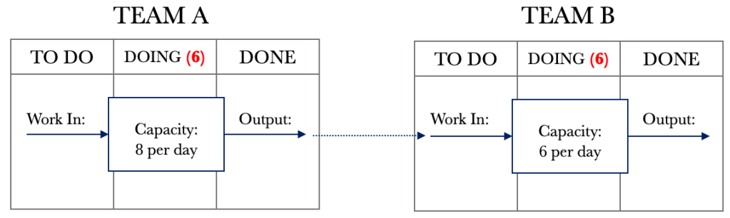
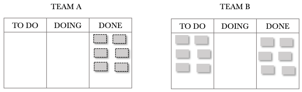
The diagram above shows that Team A can service eight requests per day and that Team B can service six requests per day. For our example, we will assume that demand exceeds capacity and that Team A will always be in a position to pull eight requests per day. With dependent Kanban boards, it is important to note that the DONE column feeds the TO DO column of the other. We could also represent the above situation on a single board, but for now, let’s consider them separate as this is a good way for us to visualise the effects of dependency.
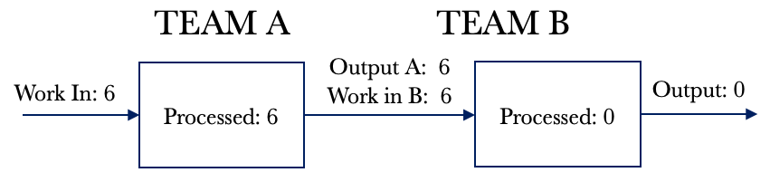
Let’s take a look at the system view of dependency. We will then work through the Kanban board. Using the example above, let’s draw out the system diagram.
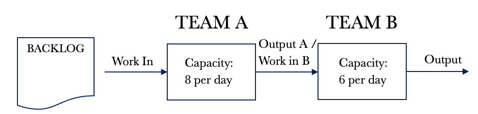
We have work that flows through the system, and the system has WIP that requires processing. Let’s look at a few days of processing for the above system with dependent events. I have added a backlog of activity to the diagram above. Currently, our demand exceeds our capacity, and we will assume we have 200 requests in the backlog to simplify tracking.
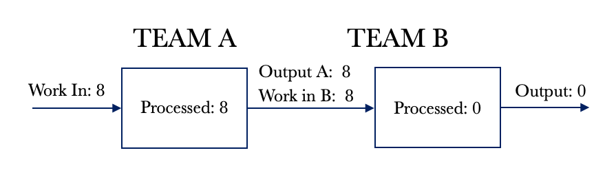
We will assume that the system is empty and that we are at day 1 of processing. For Day 1, Team A pulls eight requests from the backlog. It takes Team A a day to process their tasks, and at the end of the day, they complete eight requests. The partially completed requests are passed to Team B for processing. This flow is shown below.
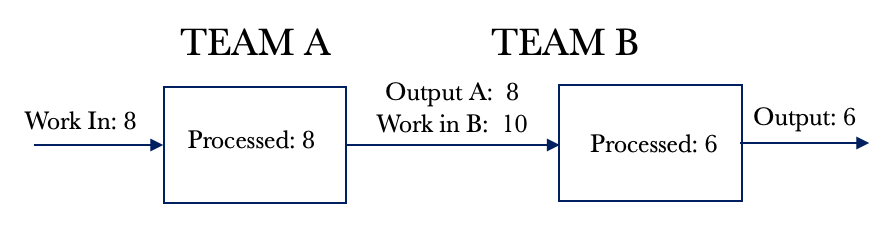
Look at Day 2 below. Team B pulls in 6 requests and fulfils these. We now have six fully serviced requests. Team A pulls another eight requests and completes their portion of the work. These requests are passed on to Team B for additional processing. We notice that the WIP for Team B has increased by 2 for the day.
Let’s look at Day 3 below. Team B pulls in 6 requests and fulfils these as per Day 2. We now have another six fully serviced requests on Day 3. Team A pulls their eight daily requests and passes them on to Team B for additional processing. We that the WIP for Team B has increased by another 2.
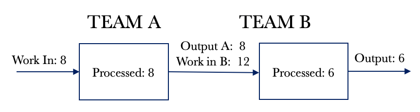
Looking at the situation above, we can see that we will fully service six requests every day we work. We will also increase our WIP by 2. We have already seen that an increase in WIP will increase cycle times. Our cycle times would continue to grow over time.
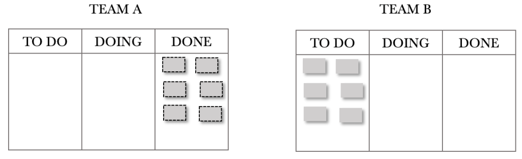
Let’s see how this plays out on the Kanban Boards. The sequence shows the first few days. For the illustration below, I have chosen not to show the 200 backlog items but instead decided to show the requests pulled through on the day. There are no requests shown in Team A’s TO DO because of this. Note that the board position shows the end of the day, so the tickets will appear in the DONE column. I want to convey the build-up of WIP we see in Team B’s TO DO. The end of Day 1 is shown below.
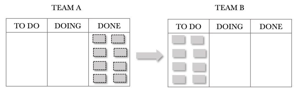
Team A and Team B’s boards above show that Team A completed their eight requests on Day one and passed these on to Team B. At the end of day 1, Team B now has eight requests in their TO DO that require final processing. They start on these requests the next day.
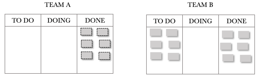
The end of Day 2 is shown below. Team A has completed another eight requests and passed these on to Team B for processing. Team B managed to complete six requests on the day. An important thing to note with dependent services is that items are finished when the last team has completed their task. The request is fulfilled once all processing for it is complete. We have so far completed six requests with a cycle time of 2 days.
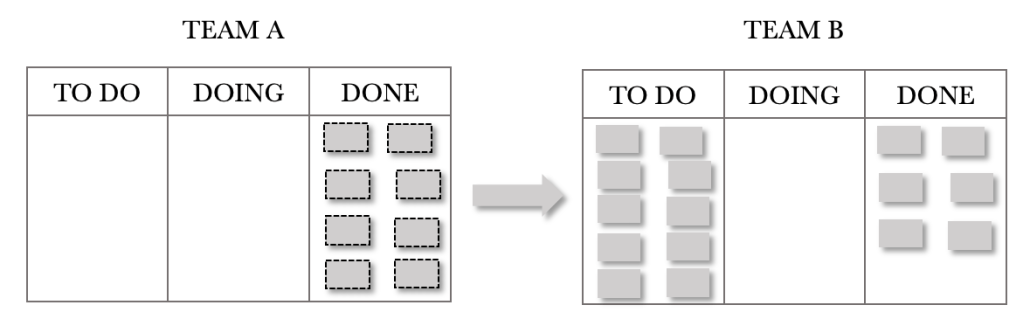
Note how Team B’s TO DO has grown by two requests. When Team B starts day 3, they would already have increased their WIP by 2. Given what we learned about the link between WIP and cycle times, it is reasonable to expect that our cycle times will increase over time. Let’s have a look at day 3.
The end of Day 3 is shown below. There is no need to describe the situation in detail as it is a repeat of the previous day. The thing we need to note is the build-up of Team B’s TO DO.
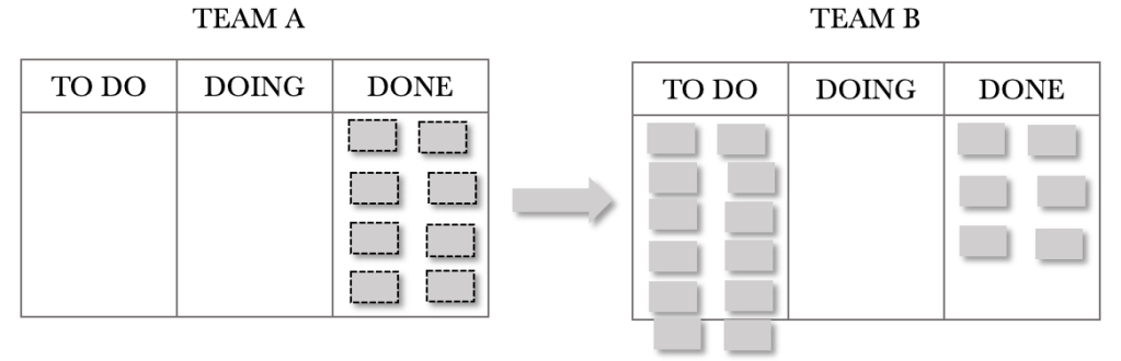
And at the end of day 4. Team B’s WIP continues to grow.

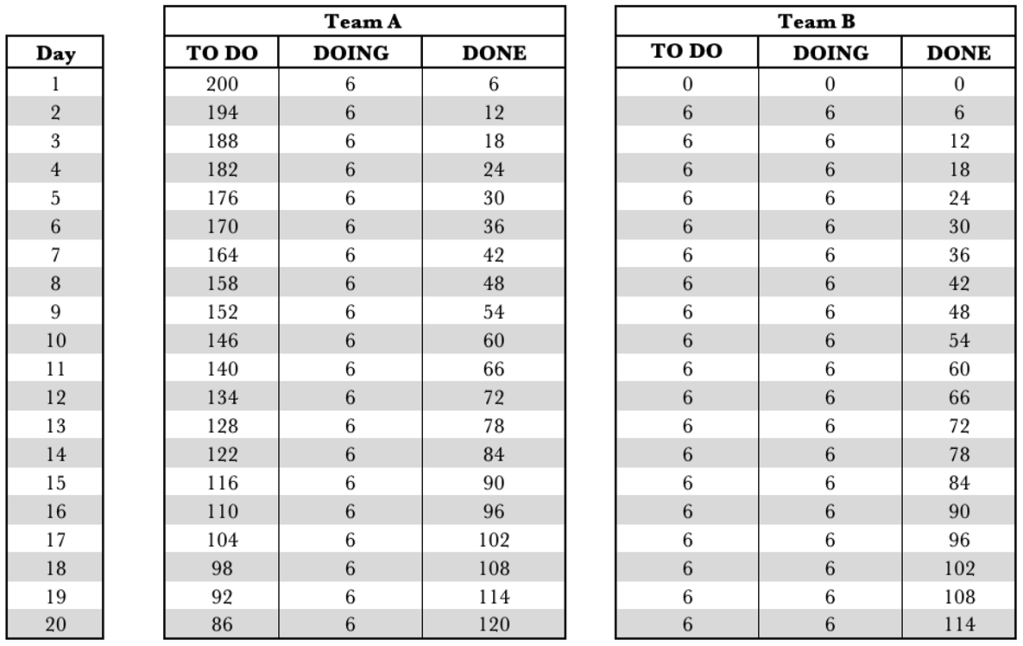
We have looked at the system view of dependency and have also looked at the Kanban boards. We have tools that can provide us with further insight. Let’s apply the CFD, Run Chart and Frequency Graph to our dependent service. Let’s take a look at our data table first.
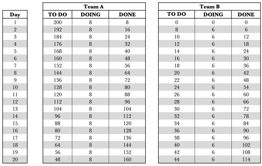
The table above shows Team B’s WIP growing by 2 per day. It also shows that over the 20 days, Team A completed 160 requests, and Team B completed 114 requests. Our overall performance for the end-to-end service was 114 requests fulfilled. With dependent systems, we have to look at the service as a whole. We cannot look at the individual performance of the components.
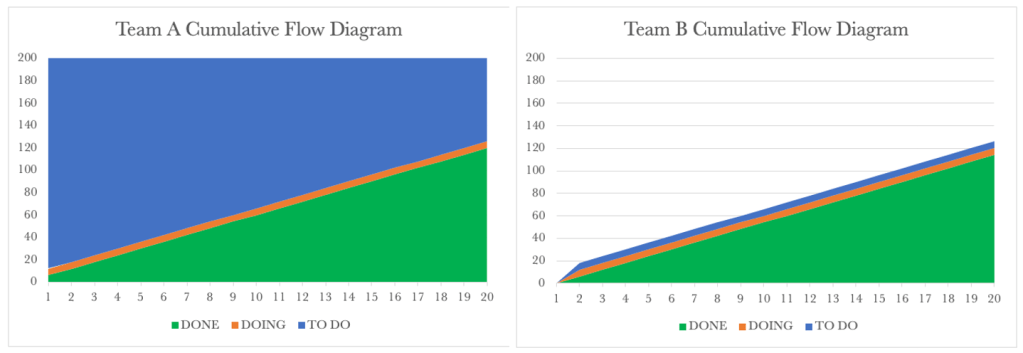
Below are the CFD’s for the two teams.
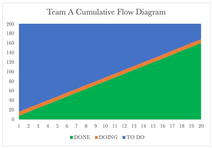
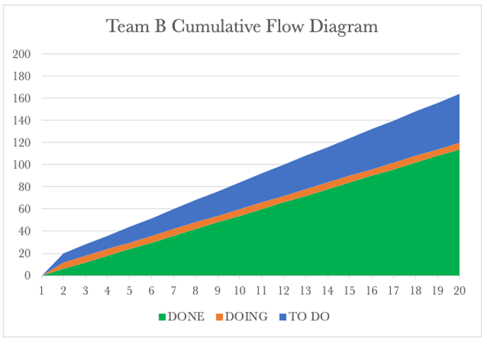
Team A’s CFD shows the burndown of the 200 requests over time. After 20 days, Team A has serviced 160 requests and passed these on to Team B.
We know that for our service, Team B governs our fulfilment rate. Looking at the Team B CFD, we see a steady output of 6 requests per day. What we also see is the continued rise of Team B’s WIP. We know that each of our tools tells a story. Let’s have a look at the Run Charts for both next.
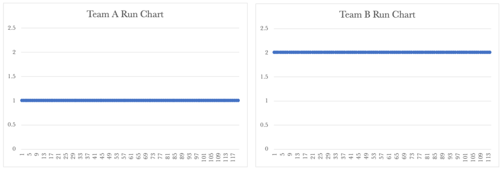
Below are the Run Charts for the two teams.
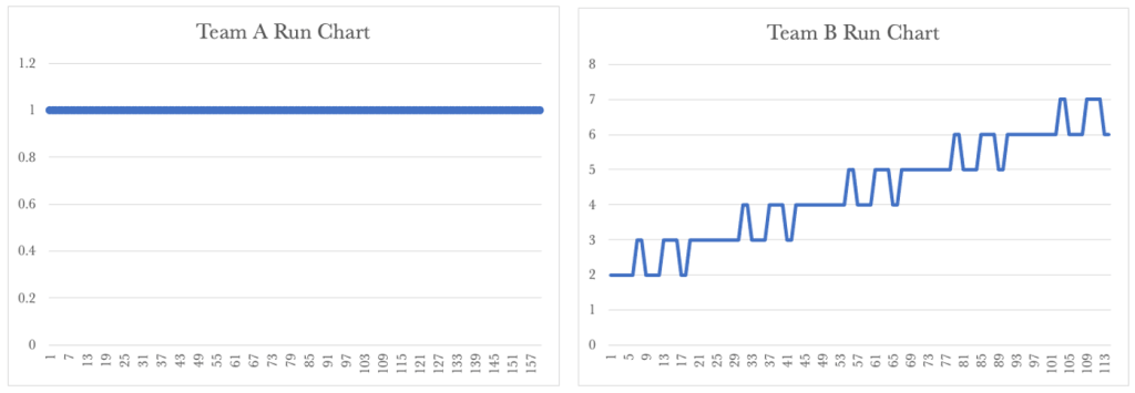
Team A’s Run Chart shows a steady cycle time of 1 day.
Team B’s run chart shows a rise in their cycle time over time. Team B’s performance governs our overall service performance, so our customers continue to see rising lead times over time. The Run Charts above show how important it is for us to take a global view of the service we provide.
Let’s have a look at the Frequency Graphs for both next.
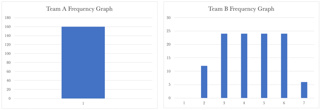
Team A’s Frequency Graph shows a steady cycle time of 1 day for their requests. Team B’s shows a wide distribution of frequency. So whilst we have part of our service stable, the other part of the service is spiralling out of control. Knowing that we need to look at the service as a whole, we have a situation that needs our attention.
Let’s have a look at how we tackle this next.
t’s go back to our Kanban boards. We had learned before that limiting WIP was essential to improve flow. We have seen above that if we limited WIP to the team’s capacity, overall, our cycle times would grow when we have dependent activities that have differing WIP limits. The important lesson here is that local optimisation may not lead to global improvements. Putting WIP limits locally, in our example, increased our cycle times. The other important lesson for us to note is that the constraint governs the output for the whole system. In our situation, the rate at which Team B can service requests governs the output for the system as a whole.

So how could we handle this situation? Mapping out the system shows that we have a constraint; Team B. One way to tackle our problem is to limit the WIP for both boards to 6, our constraint. You may initially get push back that this is unacceptable, as we will have people or resources that aren’t busy all the time. I would respond with, ‘Would you rather have longer cycle times and increased WIP or the ability to have due date predictability and improved performance?’
Let’s look at the Kanban boards below and put in a WIP limit aligned with our constraint.
Let’s walk through the first three days with a balanced WIP limit and see how this compares to our previous example. We will again assume that the system is empty and that we are at day 1 of processing. For Day 1, Team A pulls six requests from the backlog even though the team can service eight requests. The WIP limit for Team A overrides their team capacity and governs how much work can be pulled. It takes Team A a day to process their six requests, and at the end of the day, they have completed all 6. Team A passes the six partially completed requests to Team B for processing. This flow is shown below.
On day 2, Team B pulls in 6 requests and processes them. These six requests are now considered complete. Team A pulls six requests from the backlog and process these for the day. On day 2, Team A has partially serviced six requests. The interesting thing to note here is that we don’t have a build-up of WIP and so will not have the corresponding increase in cycle times. We have balanced flow and not capacity. We now have a system through which work is flowing smoothly. The days that follow day 2 are the same as day 2.
Ensuring that we release work at the rate of our constraint is essential to balancing flow. We often receive work and then pass this on without any appreciation for the upstream or downstream WIP limits. We must ensure that we map the service end to end and then put a WIP limit that matches our constraint’s capacity.
The constraint, Team B in our case, should be considered the ‘Drum’ for the system. The Drum sets the pace at which we can service requests.

Let’s use our Kanban boards to map out the first few days. We will start again with an empty system and assume that we have 200 requests in our backlog. Again, I will not be showing the 200 requests on the boards to keep the diagrams clean. Let’s start with the end of day 1.
At the end of day 1, we see that Team A has processed six requests and passed these on to Team B for processing. Fast-forwarding to Day 2, shown below, we see that Team A processed another six requests for the day, and Team B has processed their 6.
On day 2, Team B pulls in 6 requests and processes them. These six requests are now considered complete. Team A pulls six requests from the backlog and process these for the day. On day 2, Team A has partially serviced six requests. The interesting thing to note here is that we don’t have a build-up of WIP and so will not have the corresponding increase in cycle times. We have balanced flow and not capacity. We now have a system through which work is flowing smoothly. The days that follow day 2 are the same as day 2.
Let’s take a look at day 3.
Day 3 looks exactly like day 2. There is no build-up of WIP, and our requests are still flowing smoothly through the dependent system.
Leveraging our control tools again, let’s see what is happening in the system.
Let’s apply the CFD, Run Chart and Frequency Graph to our dependent service that has been WIP-limited to the rate of the constraint. Let’s take a look at our data table first.
The table above shows Team B’s WIP remains constant. It also shows that over the 20 days, Team A completed 120 requests, and Team B completed 114 requests. Team B completes the same number of requests whether we limit the WIP for Team A to the constraint or not. Our overall performance for the service was 114 requests fulfilled. Just as before, our overall performance has not dropped.
Below are the CFD’s for the two teams.
Team A’s CFD shows the burndown of the 200 requests over time. After 20 days, Team A has serviced 120 requests and passed these on to Team B.
We know that for our service, Team B governs our output. Looking at the Team B CFD, we see a steady production of 6 requests per day. We also see that Team B’s WIP remains constant. Let’s look at the Run Charts next to see how this differs from the previous example.
Team A’s Run Chart shows a steady cycle time of 1 day.
Team B’s run chart now shows a steady cycle time. Team B’s performance governs our overall service performance, and now our customers experience a consistent delivery rate. The Run Charts above show how important it is for us to take a global view of our service and show that we have managed to get work flowing smoothly with consistent due-date delivery performance.
Let’s have a look at the Frequency Graphs for both next.
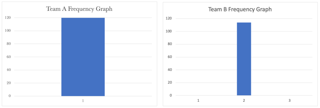
Team A’s Run Chart shows a steady cycle time of 1 day for their requests. Team B’s shows a constant frequency of 2 days. We now have a stable system, and work is flowing predictably. We can be confident that when Team A pulls work from the backlog, we will deliver it to the customer in two days.
Ensuring that we release work at the rate of our constraint is essential to balancing flow.
While we have made progress with dependent services, let’s look at what happens when we combine dependent services with variability.
